Shading alternating rows in an Excel spreadsheet is a great way to enhance the readability of your data. If you've ever done this job by manually highlighting and shading cells, you know it's tedious and your careful formatting can easily get messed up when you edit, sort and filter your data.

Here are two quick and easy ways to get shading on alternating rows that won't require you to re-do the job every time you edit the data.

1. Turn your data list into a Data Table

If your data is arranged in proper list format (a complete set of column labels in the top row followed by continuous rows of data) the simplest way to get row shading is to turn it into a Data Table. (Before you do this: You can't "share" a workbook that contains a Data Table, so if you plan to turn on sharing for your workbook, use Conditional Formatting method instead.)

To turn your list into a Data Table:

1. Click inside your data list.
2. Select Home > Format as Table (in the Styles group) and click on a format that includes row shading.
3. Confirm the boundaries of your list, and click OK.

The shading will adapt itself no matter how you edit, sort or filter your data!

2. Use Conditional Formatting

If you want to be able to share your workbook, or if your data is not suitable for changing into a Data Table, copy this convenient conditional formatting rule that tells Excel to shade every cell that's in an even-numbered row.

1. Select the area of the worksheet that you want to format.
2. Select Home > Conditional Formatting > New Rule.
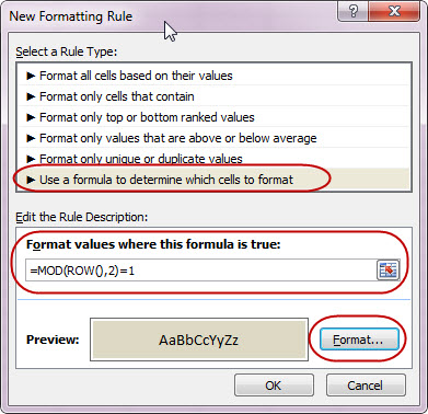
3. Under Select a Rule Type: click on "Use a formula to determine which cells to format".
4. Copy the formula below and then click in the box labelled "Format values where this formula is true" and paste  using the Ctrl+V shortcut.
   • =MOD(ROW(),2)=1
   • Include the first equals sign, but not the bullet.
   • This function checks whether the row number of a cell is evenly divisible by 2--if it is, the conditional formatting is applied to the cell. If you change the number 2 in this formula to 3, 4, or 5, you can use it to shade every 3rd, 4th, or 5th row.
5. Click on the Format... button to see the Format Cells dialogue box.
6. Click on the Fill tab and select the colour you want to use for shading.
7. Click OK  in the Format Cells dialogue.
8. Click OK in the New Formatting Rule dialogue.

 

Note: While this method works is much more reliable than manually formatting your worksheet, it's possible to lose the formatting from shaded rows if you move data around by dragging the cell's selection border. You can avoid this by using copy and paste instead of dragging to move your data. To fix this problem if it occurs to you, highlight some cells from an unaffected area, click on the Format Painter (Home ribbon, Clipboard group), then click and drag over the affected cells.

To learn more about Data Tables or Conditional Formatting, please take advantage of any of our Computer Skills Learning Resources.